原文链接: https://leetcode-cn.com/problems/minimum-cost-to-make-at-least-one-valid-path-in-a-grid

英文原文

Given a m x n grid. Each cell of the grid has a sign pointing to the next cell you should visit if you are currently in this cell. The sign of grid[i][j] can be:

• 1 which means go to the cell to the right. (i.e go from grid[i][j] to grid[i][j + 1])
• 2 which means go to the cell to the left. (i.e go from grid[i][j] to grid[i][j - 1])
• 3 which means go to the lower cell. (i.e go from grid[i][j] to grid[i + 1][j])
• 4 which means go to the upper cell. (i.e go from grid[i][j] to grid[i - 1][j])

Notice that there could be some invalid signs on the cells of the grid which points outside the grid.

You will initially start at the upper left cell (0,0). A valid path in the grid is a path which starts from the upper left cell (0,0) and ends at the bottom-right cell (m - 1, n - 1) following the signs on the grid. The valid path doesn't have to be the shortest.

You can modify the sign on a cell with cost = 1. You can modify the sign on a cell one time only.

Return the minimum cost to make the grid have at least one valid path.

 

Example 1:

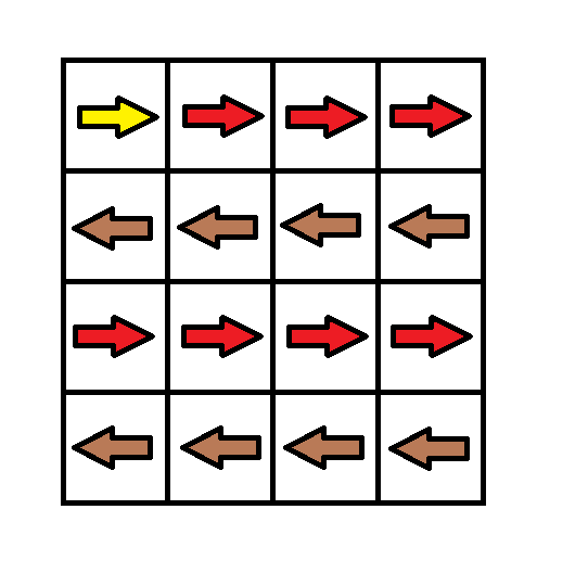
Input: grid = [[1,1,1,1],[2,2,2,2],[1,1,1,1],[2,2,2,2]]
Output: 3
Explanation: You will start at point (0, 0).
The path to (3, 3) is as follows. (0, 0) --> (0, 1) --> (0, 2) --> (0, 3) change the arrow to down with cost = 1 --> (1, 3) --> (1, 2) --> (1, 1) --> (1, 0) change the arrow to down with cost = 1 --> (2, 0) --> (2, 1) --> (2, 2) --> (2, 3) change the arrow to down with cost = 1 --> (3, 3)
The total cost = 3.

Example 2:

Input: grid = [[1,1,3],[3,2,2],[1,1,4]]
Output: 0
Explanation: You can follow the path from (0, 0) to (2, 2).

Example 3:

Input: grid = [[1,2],[4,3]]
Output: 1

Example 4:

Input: grid = [[2,2,2],[2,2,2]]
Output: 3

Example 5:

Input: grid = [[4]]
Output: 0

 

Constraints:

• m == grid.length
• n == grid[i].length
• 1 <= m, n <= 100

中文题目

给你一个 m x n 的网格图 grid 。 grid 中每个格子都有一个数字，对应着从该格子出发下一步走的方向。 grid[i][j] 中的数字可能为以下几种情况：

• 1 ，下一步往右走，也就是你会从 grid[i][j] 走到 grid[i][j + 1]
• 2 ，下一步往左走，也就是你会从 grid[i][j] 走到 grid[i][j - 1]
• 3 ，下一步往下走，也就是你会从 grid[i][j] 走到 grid[i + 1][j]
• 4 ，下一步往上走，也就是你会从 grid[i][j] 走到 grid[i - 1][j]

注意网格图中可能会有 无效数字 ，因为它们可能指向 grid 以外的区域。

一开始，你会从最左上角的格子 (0,0) 出发。我们定义一条 有效路径 为从格子 (0,0) 出发，每一步都顺着数字对应方向走，最终在最右下角的格子 (m - 1, n - 1) 结束的路径。有效路径 不需要是最短路径 。

你可以花费 cost = 1 的代价修改一个格子中的数字，但每个格子中的数字 只能修改一次 。

请你返回让网格图至少有一条有效路径的最小代价。

 

示例 1：

输入：grid = [[1,1,1,1],[2,2,2,2],[1,1,1,1],[2,2,2,2]]
输出：3
解释：你将从点 (0, 0) 出发。
到达 (3, 3) 的路径为： (0, 0) --> (0, 1) --> (0, 2) --> (0, 3) 花费代价 cost = 1 使方向向下 --> (1, 3) --> (1, 2) --> (1, 1) --> (1, 0) 花费代价 cost = 1 使方向向下 --> (2, 0) --> (2, 1) --> (2, 2) --> (2, 3) 花费代价 cost = 1 使方向向下 --> (3, 3)
总花费为 cost = 3.

示例 2：

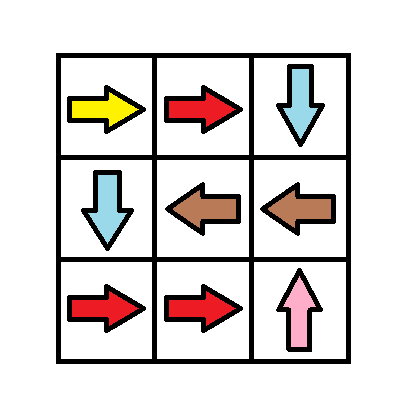
输入：grid = [[1,1,3],[3,2,2],[1,1,4]]
输出：0
解释：不修改任何数字你就可以从 (0, 0) 到达 (2, 2) 。

示例 3：

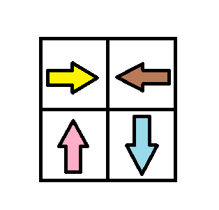
输入：grid = [[1,2],[4,3]]
输出：1

示例 4：

输入：grid = [[2,2,2],[2,2,2]]
输出：3

示例 5：

输入：grid = [[4]]
输出：0

 

提示：

• m == grid.length
• n == grid[i].length
• 1 <= m, n <= 100

通过代码

高赞题解

题目分析

虽然题目的描述中写了有效路径不需要是最短路径，但其实这道题目还是一个最短路径问题，只不过要求的最短距离并不是在网格中行走的距离，而是改变方向的次数。

所谓最短路径问题，就是对于图 $G(V,E)$，寻找从 $u\in V$ 到 $v\in V$ 的最短距离。最短路径的算法有很多，包括 Dijkstra，Floyd，Bellman-Ford，SPFA 等。

Dijkstra

Dijkstra 算法是求取单源最短路径的常用算法，其基本思想是每次用当前未拓展且具有最小权值的点来更新源点到其余顶点的距离。Dijkstra 算法的时间复杂度包含两个部分：找到最小节点并将其移除的用时 $T_{extract_min}$，以及更新某一节点权值的用时 $T_{decrease_key}$。因为每个节点最多充当一次最小节点，而每条边最多参与一次更新，算法整体的时间复杂度可以表示为
$$\Theta(V)\cdot T_{extract_min}+\Theta(E)\cdot T_{decrease_key}$$

数据结构	$T_{extract_min}$	$T_{decrease_key}$	总时间复杂度
数组	$O(V)$	$O(1)$	$O(V^2+E)$
优先队列（小根堆）	$O(\log V)$	$O(\log V)$	$O((V+E)\log V)$
Fibonacci堆	均摊$O(\log V)$	均摊$O(1)$	均摊$O(V\log V + E)$

由于 Fibonacci 堆实现较为复杂，各语言标准库未提供实现（C++ 的 Boost 库实现了这一数据结构），并且其实际运行效率与优先队列相比的优势并不明显，所以基于优先队列的实现是 Dijkstra 算法最常见的实现方式。

需要注意的是，Dijkstra 算法在图中存在负环的情况下不适用！对于无向图来说，只要有一条负边，就构成了一个两节点的负环，所以在无向图中只要有负边就不能使用 Dijkstra 算法。

参考实现 （108ms）

[]
const int dx[5] = {0, 1, -1, 0, 0};
const int dy[5] = {0, 0, 0, 1, -1};
const int INF = 0x3f3f3f3f;
typedef pair<int, int> pii;

class Solution {
public:
    int minCost(vector<vector<int>>& grid) {
        int n = grid.size(), m = grid[0].size();
        vector<vector<int>> dist(n, vector<int>(m, INF));
        dist[0][0] = 0;
        priority_queue<pii, vector<pii>, greater<>> pq;
        pq.push(make_pair(0, 0));
        vector<bool> vis(n * m);
        while (!pq.empty()) {
            pii f = pq.top();
            pq.pop();
            if (vis[f.second]) continue;
            vis[f.second] = true;
            int y = f.second / m, x = f.second % m;
            for (int k = 1; k <= 4; ++k) {
                int nx = x + dx[k], ny = y + dy[k];
                if (nx < 0 || nx >= m || ny < 0 || ny >= n)
                    continue;
                int nd = f.first + (grid[y][x] == k ? 0 : 1);
                if (nd < dist[ny][nx]) {
                    dist[ny][nx] = nd;
                    pq.push(make_pair(dist[ny][nx], ny * m + nx));
                }
            }
        }
        return dist[n - 1][m - 1];
    }
};

代码解析

在优先队列实现中，并不需要显式地进行 $decrease_key$ 操作，因为我们只要将更新后的权值加入优先队列中，它就会排到原先较大的权值前面，从而变相实现了权值的减小。而由于我们使用了标记数组 vis 来记录每一个节点是否已经拓展过，原来较大的权值在出队时就会被跳过。

BFS

对于 BFS，相信大家一定都很熟悉了。与 DFS 相比，BFS 的特点是按层遍历，从而可以保证首先找到最优解（最少步数、最小深度）。从这个意义上讲，BFS 解决的其实也是最短路径问题。这一问题对应的图 $G$ 包含的所有顶点即为状态空间，而每一个可能的状态转移都代表了一条边。

比如，在经典的迷宫问题中，每一个状态 $(x,y)$ 代表了一个顶点，而一个无障碍格子与其相邻的无障碍格子之间则存在一条无向边。

那么，这个图 $G$ 和一般的图相比，有什么特点呢？

关键就在于边的权值。在 BFS 问题中，所有边的权值均为 1！因为我们每一次从一个状态转移到一个新的状态，就多走了一步。正因为边权值均为 1，我们用一个队列记录所有状态，前面的状态对应的总权值一定小于后面的状态，所以我们就可以在 $O(1)$ 的时间内实现找到最小节点并将其移除的操作（只要取队头，然后出队就可以了），从而寻找最短路径的时间复杂度就减小到了 $O(V+E)$。

但普通的 BFS 算法，在本题中并不适用，因为存在权值为 0 的边！如果从一个格子到另一个格子，不需要修改格子上的标记，那么这一步移动的权值就为 0。如果我们还沿用普通 BFS 的做法，就无法保证队头元素一定是当前具有最小权值的节点。

怎么办呢？简单粗暴的做法是：允许多次扩展同一个点。只要当前边能够更新节点的权值，就将节点再次入队。

参考实现 （92ms）

[]
const int dx[5] = {0, 1, -1, 0, 0};
const int dy[5] = {0, 0, 0, 1, -1};
const int INF = 0x3f3f3f3f;
typedef pair<int, int> pii;

class Solution {
public:
    int minCost(vector<vector<int>>& grid) {
        int n = grid.size(), m = grid[0].size();
        queue<pii> pq;
        pq.push(make_pair(0, 0));
        vector<vector<int>> dist(n, vector<int>(m, INF));
        dist[0][0] = 0;
        while (!pq.empty()) {
            pii f = pq.front();
            pq.pop();
            int y = f.first, x = f.second;
            for (int k = 1; k <= 4; ++k) {
                int nx = x + dx[k], ny = y + dy[k];
                if (nx < 0 || nx >= m || ny < 0 || ny >= n)
                    continue;
                int nd = dist[y][x] + (grid[y][x] == k ? 0 : 1);
                if (nd < dist[ny][nx]) {
                    dist[ny][nx] = nd;
                    pq.push(make_pair(ny, nx));
                }
            }
        }
        return dist[n - 1][m - 1];
    }
};

SPFA

如果一个节点已经在队列中，其实就没有必要将其再次入队了。这是 SPFA 算法的基本思想。可以看到，与上面的BFS 方法相比，就是增加了一个 in 数组来判断当前节点是否已经在队列中。

SPFA 算法是一个十分依赖于数据的算法。在特定的数据下，SPFA 会退化为 Bellman-Ford，时间复杂度为 $O(V\cdot E)$。一般的编程竞赛中，涉及到最短路径的题目，都会有专门卡SPFA的数据，所以一般情况下还是使用 Dijkstra 算法。本题的测试数据相对较弱，BFS 和 SPFA 都可以顺利通过，甚至 SPFA 的运行时间还要长于 BFS（修改 in 数组状态带来了额外的开销）。

SPFA 的好处是可以判断负环。我们可以用一个数组记录每个顶点的入队次数，如果有顶点的入队次数超过了 $V$ 次，则代表图中存在负环。

参考实现 （120ms）

[]
const int dx[5] = {0, 1, -1, 0, 0};
const int dy[5] = {0, 0, 0, 1, -1};
const int INF = 0x3f3f3f3f;
typedef pair<int, int> pii;

class Solution {
public:
    int minCost(vector<vector<int>>& grid) {
        int n = grid.size(), m = grid[0].size();
        queue<pii> pq;
        pq.push(make_pair(0, 0));
        vector<vector<bool>> in(n, vector<bool>(m));
        vector<vector<int>> dist(n, vector<int>(m, INF));
        dist[0][0] = 0;
        in[0][0] = true;
        while (!pq.empty()) {
            pii f = pq.front();
            pq.pop();
            int y = f.first, x = f.second;
            in[y][x] = false;
            for (int k = 1; k <= 4; ++k) {
                int nx = x + dx[k], ny = y + dy[k];
                if (nx < 0 || nx >= m || ny < 0 || ny >= n)
                    continue;
                int nd = dist[y][x] + (grid[y][x] == k ? 0 : 1);
                if (nd < dist[ny][nx]) {
                    dist[ny][nx] = nd;
                    if (!in[ny][nx]) {
                        pq.push(make_pair(ny, nx));
                        in[ny][nx] = true;                                          
                    }
                }
            }
        }
        return dist[n - 1][m - 1];
    }
};

0-1 BFS

说了这么多，本题的最优方法是什么呢？我们需要注意到，本题中的权值如果不为 1，就一定为 0。如何利用这一特殊性质，在节点不重复入队的情况下，保证队头元素始终是最小权值的节点？

如果某条边权值为 0，那么新拓展出的节点权值就和当前队头节点权值相同，也就自然可以作为下一次拓展的起点，所以，我们需要把它放在队头。而如果某条边的权值为 1，我们就把它正常地放在队尾。怎样实现这一操作？

双端队列，也就是 Deque，在此时就有了用武之地。它可以在 $O(1)$ 时间内从头或尾插入或删除节点，刚好满足了我们的需要。

参考实现 （48ms）

[]
const int dx[5] = {0, 1, -1, 0, 0};
const int dy[5] = {0, 0, 0, 1, -1};
typedef pair<int, int> pii;

class Solution {
public:
    int minCost(vector<vector<int>>& grid) {
        int n = grid.size(), m = grid[0].size();
        deque<pii> pq;
        pq.push_back(make_pair(0, 0));
        vector<vector<bool>> vis(n, vector<bool>(m));
        while (!pq.empty()) {
            pii f = pq.front();
            pq.pop_front();
            int y = f.second / m, x = f.second % m;
            if (vis[y][x]) continue;
            vis[y][x] = true;
            if (y == n - 1 && x == m - 1)
                return f.first;
            for (int k = 1; k <= 4; ++k) {
                int nx = x + dx[k], ny = y + dy[k];
                if (nx < 0 || nx >= m || ny < 0 || ny >= n)
                    continue;
                if (grid[y][x] == k) 
                    pq.push_front(make_pair(f.first, ny * m + nx));
                else
                    pq.push_back(make_pair(f.first + 1, ny * m + nx));
            }
        }
        return 0;
    }
};

统计信息

通过次数	提交次数	AC比率
3820	7167	53.3%

提交历史

提交时间	提交结果	执行时间	内存消耗	语言